Implementation

In this section, you can find an overview about the implementation and the results of the calibration engine.

Data

The dataset contains 2434 measurements, where each measurement is composed by:

$time$: $\space$ timestamp of the actual measurements;
$tick\_steer$: $\space$ reading tick of the absolute encoder for the steering angle of the front wheel;
$tick\_traction$: $\space$ reading tick of the incremental encoder for the traction of the front wheel;
$model\_pose$: $\space$ [$x_m$,$y_m$,$\theta_m$] 3x1 vector representing the odometry of the robot (2D translation + orientation);
$tracker\_pose$: $\space$ [$x_t$,$y_t$,$\theta_t$] 3x1 vector representing the ground truth 2D pose of the sensor (2D translation + orientation);

Parameters to calibrate

Parameters must be calibrated are the kinematic parameters of the robot and sensor pose (position and orientation) with respect to kinematic center of the robot. In detail:

$k_s$: $\space$ how many radians correspond to one tick;
$k_t$: $\space$ how many meters correspond to one tick;
$\delta_{offset}$: $\space$ at which angle corresponds the zero of the wheel;
$a$: $\space$ the lenght of the baseline;
$v_{sensor}^{robot}$: $\space$ sensor pose [$x$, $y$, $\theta$] relative to the robot.

Thus, in total the parameters to calibrate are 7.

Kinematic model

The kinematic model of the front-traction wheel tricycle is the following:

$$ \begin{cases} dx = s \cos(\delta)\cos(d\theta) \\ dy = s \cos(\delta)\sin(d\theta) \\ d\theta = s \frac{\sin(\delta)}{a} \end{cases} $$

where:

$\delta$: steering angle of the front wheel
$s$: distance traveled from tricycle
$a$: length of the baseline

The kinematic model of the robot is expressed with respect to its kinematic center.

Algorithm

Calibration cycle is executed multiple times. A threshold is initialized to 9999 in order to select all samples in the first calibration cycle. In the next cycles it is updated to remove the worst samples for the calibration. Each cycle is composed by the following steps.

Initialization step

Tricycle and sensor poses are set equal to $model\_pose$ and $tracker\_pose$ of the first measurement. Also the ticks about steering angle and traction are initialized with $tick\_steer$ and $tick\_traction$ of the first measurement.
Finally, given that the number of parameters to calibrate is 7, two matrices $\textbf{H}$ (7x7 matrix) and $\textbf{b}$ (7x1 matrix) are initialized to zero; also variable $total\_error$ is initialized to zero.

Update step

Given the measurement $i$-th, the following information are saved to compute the prediciton:

\[(tick\_steer_i, tick\_traction_i, tick\_traction_{i+1})\]

Then, the following steps are executed

$$ $$

Prediction step :
Firstly, encoder ticks are converted into steering angle and traveled distance. Starting with the steering angle $\delta$:
\[\delta = \begin{cases} \frac{2\pi}{max\_steer}\cdot(tick\_steer_i - max\_steer) \cdot k_s , & \text{if } tick\_steer_i > \frac{max\_steer}{2} \\ \frac{2\pi}{max\_steer}\cdot tick\_steer_i \cdot k_s, & \text{otherwise} \\ \end{cases}\]
After this, the offset must be added to $\delta$:
\[\delta = \delta + \delta_{offset}\]
For the traction distance $s$:
\[\Delta ticks = tick\_traction_{i+1} - tick\_traction_i \\ s = k_t \cdot \frac{\Delta ticks}{max\_traction}\]
At this point, the robot displacement $v_{dRobot}$ can be predicted through the kinematic model. The sensor displacement can be computed using the static matrix product:

$$ T_{dSensor} = v2t(v_{sensor}^{robot})^{-1} \cdot v2t(v_{dRobot}) \cdot v2t(v_{sensor}^{robot}) $$

where $v2t$ is a function that converts a pose $[x, y, \theta]$ in a homogeneous matrix. Finally, the robot and sensor poses can be updated:
\[\begin{equation} v_{next\_robot} = t2v(v2t(v_{robot}) \cdot v2t(v_{dRobot})) \\ v_{next\_sensor} = t2v(v2t(v_{sensor}) \cdot T_{dSensor}) \\ v_{robot} = v_{next\_robot} \\ v_{sensor} = v_{next\_sensor} \end{equation}\]
where $t2v$ is a function to convert a homogeneous matrix in a pose $[x, y, \theta]$
Computation of the error:
The prediction is the displacement of the sensor $T_{dSensor}$ computed in the prediction step.
The observation is the displacement between the $tracker\_pose_i$ and the next tracker pose $tracker\_pose_{i+1}$:
\[T_{obs} = v2t(tracker\_pose_i)^{-1} \cdot v2t(tracker\_pose_{i+1})\]
The error $e$ is computed as:
\[e = t2v(T_{obs}^{-1} \cdot T_{dSensor})\]
and its norm is added to $total\_error$:
\[total\_error = total\_error + \vert\vert{e}\vert\vert\]
If the error norm is higher than the threshold, discard the i-th sample.
Computation of Jacobian matrix:
Define with $f$ the entire prediction step, which takes as input the kinematic parameters and the sensor pose relative to the robot $v^{robot}_{sensor}$, and returns in output the displacement of the sensor $T_{dSensor}$. The jacobian matrix $J$ of the prediction function is a 3x7 matrix divided in:
\[J = [J_{kin} | J_{sensor}]\]
where:
- $J_{kin}$ is 3x4 matrix and concerns the kinematic parameters of the robot $params_{kin} = (k_s, k_t, \delta_{offset}, a)$. It is computed using numeric derivatives, where each column of the jacobian is computed as:
  \[J_{kin}^i = \left[\frac{t2v(f(params_{kin} + \epsilon_i, v^{robot}_{sensor})) - t2v(f(params_{kin} - \epsilon_i, v^{robot}_{sensor}))}{2\epsilon}\right]\]
  where $\epsilon_i$ is a small factor ($10^{-11}$) added only to the i-th kinematic parameters. Its value has been chosen because the smaller displacement of the robot in the dataset (along one direction) is in the order of $10^{-9}$;
- $J_{sensor}$ is a 3x3 matrix and concerns the sensor pose relative to the robot $v^{robot}_{sensor}$. It is also computed using numeric derivatives, where each column of the jacobian is computed as:
  \[J_{sensor}^i = \left[\frac{t2v(f(params_{kin}, v^{robot}_{sensor} + \epsilon_i)) - t2v(f(params_{kin}, v^{robot}_{sensor} - \epsilon_i))}{2\epsilon}\right]\]
  where $\epsilon_i$ in this case is a 3D vector that has all zeros but the i-th component which has $\epsilon$. The summation and the difference between $v^{robot}_{sensor}$ and $\epsilon_i$ is in a manifold space, so they have to be computed in the following way:
  \[v^{robot}_{sensor} + \epsilon_i = t2v(v2t(\epsilon_i) \cdot v2t(v^{robot}_{sensor})) \\ v^{robot}_{sensor} - \epsilon_i = t2v(v2t(-\epsilon_i) \cdot v2t(v^{robot}_{sensor}))\]

Now the error and the jacobian can be accumulated in the $H$ and $b$ matrices:

\[H = H + J^T \cdot J \\ b = b + J^T \cdot e\]

and the update step is executed on the entire dataset.

Regularization

L2 regularization is applied on the $H$ matrix, with $\lambda = 0.5$:

\[H = H + \lambda I_{7x7}\]

Calibration

At this point, the threshold is set equals to the mean total error accumulated during the update steps:

\[threshold = \frac{total\_error}{size_{dataset}}\]

and the linear system is solved:

\[dx \leftarrow solve(H \Delta x = -b)\]

The calibration vector $dx$ has 7 components, one for each parameters to calibrate. It is composed by:

\[dx = [dx_{kin} | dx_{sensor}]\]

where $dx_{kin}$ concerns the kinematic parameters and $dx_{sensor}$ concerns the sensor pose relative to the robot. So, for the former the calibration is a simple sum because they are in an Euclidean space: $params_{kin} = params_{kin} + dx_{kin}$

The latter is a 3D vector representing:

\[dv_{sensor}^{robot} = [dx, dy, d\theta]_{sensor}^{robot}\]

The sensor pose relative to the robot lies on a manifold, so its calibration is:

\[v_{sensor}^{robot} = t2v(v2t(dv_{sensor}^{robot}) \cdot v2t(v_{sensor}^{robot}))\]

Results

The Gauss-Newton method is run 7 times, because it has been tested to achieve the best parameters configuration. As explained in the previous section, in the first cycle the entire dataset is used for the calibration. Then, a sumbsampling of the dataset is actuated, putting a threshold for the error norm equals to the mean of the total error accumulated in the previous cycle.
In the end, the calibrated parameters are:

k_steer: 0.556352;
k_traction: 0.00947317;
steer_offset: -0.0506322;
base_line: 1.35205;
sensor_pose_rel: (1.58809, 0.0039371, 0.0163697).

The calibrated, uncalibrated and ground truth trajectories are shown below:

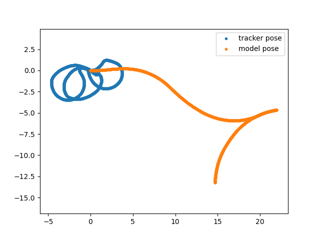Dataset model pose - Dataset tracker pose	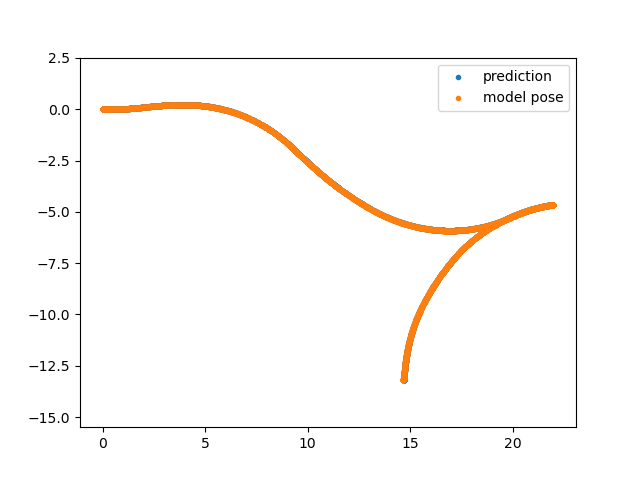Dataset model pose - Uncalibrated robot pose
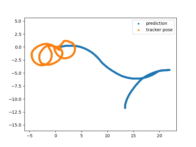Dataset tracker pose - Uncalibrated sensor pose	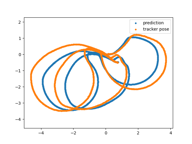Dataset tracker pose - Calibrated sensor pose

Tricycle calibration

Front-traction tricycle calibration using least-squares approach.